

Numerical Methods for Describing Data
Data can be described numerically by various statistics, or statistical measures. These statistical measures are often grouped in three categories: measures of central tendency, measures of position, and measures of dispersion.
In these lessons, we wll learn Measures of Central Tendency, Measures of Position and Measures of Dispersion.
Measures of Central Tendency
Measures of central tendency indicate the “center” of the data along the number line and are usually reported as values that represent the data.
There are three common measures of central tendency:
(i) the arithmetic mean—usually called the average or simply the mean,
(ii) the median, and
(iii) the mode.
To calculate the mean of n numbers, take the sum of the n numbers and divide it by n.
The mean can be affected by just a few values that lie far above or below the rest of the data, because
these values contribute directly to the sum of the data and therefore to the mean. By contrast, the median is a measure of central tendency that is fairly unaffected by unusually high or low values relative to the
rest of the data.
To calculate the median of n numbers, first order the numbers from least to greatest. If n is odd, then the
median is the middle number in the ordered list of numbers. If n is even, then there are two middle
numbers, and the median is the average of these two numbers.
The median, as the “middle value” of an ordered list of numbers, divides the list into roughly two equal parts. However, if the median is equal to one of the data values and it is repeated in the list, then the numbers of data above and below the median may be rather different.
The mode of a list of numbers is the number that occurs most frequently in the list.
Measures of Central Tendency - Mean, Median and Mode
This video explains how to find the measures of central tendency, which are mean, median and mode.
Measures of Position
The three most basic positions, or locations, in a list of data ordered from least to greatest are the beginning, the end, and the middle. It is useful here to label these as L for the least, G for the greatest, and M for the median. Aside from these, the most common measures of position are quartiles and percentiles. Like the median M, quartiles and percentiles are numbers that divide the data into roughly equal groups after the data have been ordered from the least value L to the greatest value G. There are three quartile numbers that divide the data into four roughly equal groups, and there are 99 percentile numbers that divide the data into 100 roughly equal groups. As with the mean and median, the quartiles and percentiles may or may not themselves be values in the data.The first quartile Q1, the second quartile Q2 (which is simply the median M), and the third quartile Q3, divide a group of data into four roughly equal groups as follows. After the data are listed in increasing order, the first group consists of the data from L to Q1, the second group is from Q1 to M, the third group is from M to Q3 and the fourth group is from Q3 to G. Because the number of data in a list may not be divisible by 4, there are various rules to determine the exact values of and , and some statisticians use different rules, but in all cases We use perhaps the most common rule, in which divides the data into two equal partsthe lesser numbers and the greater numbersand then is the median of the lesser numbers and is the median of the greater numbers.
Percentiles are mostly used for very large lists of numerical data ordered from least to greatest. Instead of dividing the data into four groups, the 99 percentiles, P1, P2, P3, ..., P99 divide the data into 100 groups. Consequently, Q1 = P25, M = Q2 = P50 and Q3 = P75. Because the number of data in a list may not be divisible by 100, statisticians apply various rules to determine values of percentiles.
Measures of Dispersion
Measures of dispersion indicate the degree of spread of the data. The most common statistics used as measures of dispersion are the range, the interquartile range, and the standard deviation. These statistics measure the spread of the data in different ways.The range of the numbers in a group of data is the difference between the greatest number G in the data and the least number L in the data, that is, G - L.
The simplicity of the range is useful in that it reflects that maximum spread of the data. However, sometimes a data value is so unusually small or so unusually large in comparison with the rest of the data that it is viewed with suspicion when the data are analyzedthe value could be erroneous or accidental in nature. Such data are called outliers because they lie so far out that in most cases, they are ignored when analyzing the data. Unfortunately, the range is directly affected by outliers.
A measure of dispersion that is not affected by outliers is the interquartile range. It is defined as the difference between the third quartile and the first quartile, that is, Q3 - Q1. Thus, the interquartile range measures the spread of the middle half of the data.
One way to summarize a group of numerical data and to illustrate its center and spread is to use the five numbers L, and G. These five numbers can be plotted along a number line to show where the four quartile groups lie. Such plots are called boxplots or box-and-whisker plots, because a box is used to identify each of the two middle quartile groups of data, and whiskers extend outward from the boxes to the least and greatest values.
This video explains the measures of position, quartiles, interquartile range, box-and-whisker plots.
Unlike the range and the interquartile range, the standard deviation is a measure of spread that depends on each number in the list. Using the mean as the center of the data, the standard deviation takes into account how much each value differs from the mean and then takes a type of average of these differences. As a result, the more the data are spread away from the mean, the greater the standard deviation; and the more the data are clustered around the mean, the lesser the standard deviation.
The standard deviation of a group of n numerical data is computed by
(1) calculating the mean of the n values,
(2) finding the difference between the mean and each of the n values,
(3) squaring each of the differences,
(4) finding the average of the n squared differences, and
(5) taking the nonnegative square root of the average squared difference.
Note on terminology: The term standard deviation defined above is slightly different from another measure of dispersion, the sample standard deviation. The latter term is qualified with the word sample and is computed by dividing the sum of the squared differences by n - 1 instead of n. The sample standard deviation is only slightly different from the standard deviation but is preferred for technical reasons for a sample of data that is taken from a larger population of data. Sometimes the standard deviation is called the population standard deviation to help distinguish it from the sample standard deviation.
This video shows how to calculate the sample standard deviation and sample variance.
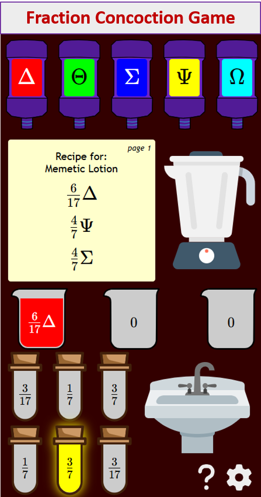
Try out our new and fun Fraction Concoction Game.
Add and subtract fractions to make exciting fraction concoctions following a recipe. There are four levels of difficulty: Easy, medium, hard and insane. Practice the basics of fraction addition and subtraction or challenge yourself with the insane level.
We welcome your feedback, comments and questions about this site or page. Please submit your feedback or enquiries via our Feedback page.


